TransferCredit.org Guide to AP® Calculus AB

This is one of the two heaviest units. You use f′ and f″ to find where a function rises, falls and bends, to locate and justify its extreme values, and to solve optimization problems. The Mean Value and Extreme Value Theorems tell you when such points must exist.

Key terms, with examples

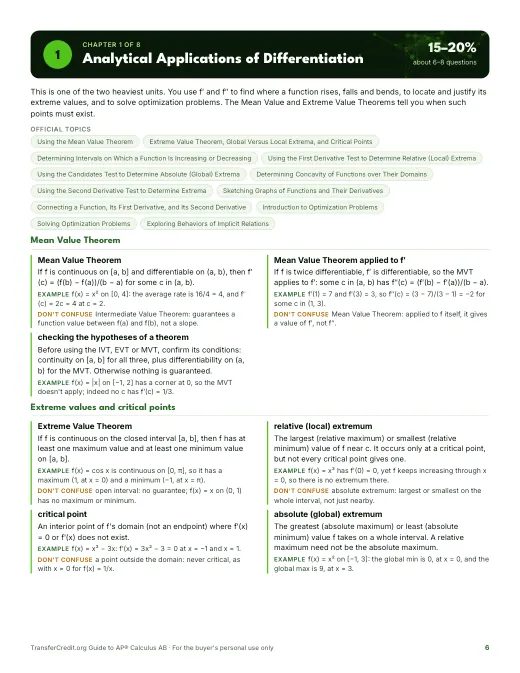
Mean Value Theorem

If f is continuous on [a, b] and differentiable on (a, b), then f′(c) = (f(b) − f(a))/(b − a) for some c in (a, b).

Example: f(x) = x² on [0, 4]: the average rate is 16/4 = 4, and f′(c) = 2c = 4 at c = 2.

Extreme Value Theorem

If f is continuous on the closed interval [a, b], then f has at least one maximum value and at least one minimum value on [a, b].

Example: f(x) = cos x is continuous on [0, π], so it has a maximum (1, at x = 0) and a minimum (−1, at x = π).

increasing and decreasing test

On an interval, if f′(x) > 0 then f is increasing; if f′(x) < 0 then f is decreasing.

Example: f(x) = x² − 6x: f′(x) = 2x − 6 < 0 for x < 3, so f decreases on (−∞, 3).

Candidates Test

For absolute extrema of a continuous f on [a, b], evaluate f at the critical points and both endpoints. The largest value is the maximum; the smallest is the minimum.

Example: f(x) = x³ − 3x on [0, 2]: f(0) = 0, f(1) = −2, f(2) = 2, so the maximum is 2 and the minimum −2.

concave up and concave down

The graph of f is concave up on an open interval where f′ is increasing (bending like a cup) and concave down where f′ is decreasing.

Example: f(x) = x³: f′(x) = 3x² decreases for x < 0 and increases for x > 0, so f is concave down, then up.

reading the graph of f′

Where the graph of f′ is above the x-axis, f is increasing; below, f is decreasing. Where f′ crosses the x-axis, f has a relative extremum.

Example: If the graph of f′ crosses the x-axis from above to below at x = 4, f has a relative maximum at x = 4.

optimization

Using the derivative to find the maximum or minimum value of a quantity, such as an area, a cost or a distance, on an interval.

Example: A rectangle with perimeter 20 has area A = x(10 − x); A′ = 10 − 2x = 0 at x = 5, so the largest area is 25.

critical points of an implicit relation

Points on the curve where dy/dx is 0 or undefined. Find them from the formula for dy/dx, keeping only points that lie on the curve.

Example: x² − y² = 9: dy/dx = x/y. No point on the curve has x = 0, so the only critical points are (±3, 0).

checking the hypotheses of a theorem

Before using the IVT, EVT or MVT, confirm its conditions: continuity on [a, b] for all three, plus differentiability on (a, b) for the MVT. Otherwise nothing is guaranteed.

Example: f(x) = |x| on [−1, 2] has a corner at 0, so the MVT doesn't apply; indeed no c has f′(c) = 1/3.

critical point

An interior point of f's domain (not an endpoint) where f′(x) = 0 or f′(x) does not exist.

Example: f(x) = x³ − 3x: f′(x) = 3x² − 3 = 0 at x = −1 and x = 1.

sign chart for f′

A number line showing where f′ is positive or negative. Mark the critical points, then test one x-value in each interval between them.

Example: f′(x) = (x − 1)(x − 4): f′(0) > 0, f′(2) < 0, f′(5) > 0, so f rises, falls, then rises.

endpoints as candidates

On a closed interval, an absolute extremum can sit at an endpoint even though f′ is not 0 there. Always evaluate f at both endpoints.

Example: f(x) = 2x + 1 on [0, 5] has no critical points; its maximum is f(5) = 11, at an endpoint.

What this area covers

How the exam asks it

Questions give a formula for f or f′, a graph of f′ described in words, or a table of derivative values, and ask where f has a relative extremum, a point of inflection or its absolute maximum. Many ask which statement must be true, so check each theorem's hypotheses before using it. Optimization items describe a fence, a box or a cost and ask for a dimension or the best value. Free-response parts ask you to justify: name the derivative and its sign change.

Common traps

Trap 1. Reading a graph of f′ as if it were the graph of f. On a graph of f′, the x-intercepts are critical points of f, and the peaks and valleys are inflection points of f.

Trap 2. Calling a point an inflection point just because f″ = 0 there. Confirm that f″ changes sign there, so that f′ switches between increasing and decreasing.

Trap 3. Stopping at the critical points when the question asks for an absolute maximum on a closed interval. An endpoint value can be larger.

Memory trick

Concave up holds water like a cup (f″ > 0); concave down spills it like a frown (f″ < 0).

Mean Value Theorem: "somewhere, the tangent is parallel to the secant."

This unit runs differentiation backward. It starts with the area under a rate graph as accumulated change, approximates that area with Riemann and trapezoidal sums, and then makes it exact with the definite integral and the Fundamental Theorem of Calculus. It ends with antiderivative rules and substitution, which every later unit uses.

Key terms, with examples

accumulation of change

The area between the graph of a rate of change and the x-axis gives the accumulated change. A positive rate gives a positive change; a negative rate, a negative change.

Example: Water flows in at a constant 4 liters per minute for 5 minutes: the area 4·5 = 20 liters is the water added.

summation notation

Σ from k = 1 to n of aₖ means a₁ + a₂ + … + aₙ. The index k counts the terms; Riemann sums are written this way.

Example: Σ from k = 1 to 4 of 2k = 2 + 4 + 6 + 8 = 20.

accumulation function

A function defined by an integral with a variable upper limit: g(x) = ∫ from a to x of f(t) dt, the accumulated signed area from a to x.

Example: g(x) = ∫ from 0 to x of 2t dt = x², so g(3) = 9.

indefinite integral and constant of integration

∫ f(x) dx = F(x) + C stands for every antiderivative of f at once, where F′(x) = f(x) and C is any constant.

Example: ∫ 6x dx = 3x² + C; with C = 2, 3x² + 2 is one particular antiderivative.

u-substitution

Reverses the chain rule. Let u be an inner function whose derivative also appears in the integrand: ∫ f(g(x))·g′(x) dx = ∫ f(u) du, with u = g(x).

Example: ∫ 2x(x² + 1)⁴ dx: u = x² + 1, du = 2x dx, so it is ∫ u⁴ du = (x² + 1)⁵/5 + C.

units of accumulated change

The unit of the area under a rate graph is the rate's unit times the input's unit: (units per hour) × hours = units.

Example: If r(t) is in gallons per hour and t is in hours, then ∫ from 0 to 3 of r(t) dt is in gallons.

definite integral

∫ from a to b of f(x) dx is the limit of Riemann sums Σ f(xₖ*)·Δxₖ as the subinterval widths shrink to 0. It gives signed area.

Example: Right sums for ∫ from 0 to 1 of x dx approach 1/2 as n grows: 0.75 (n = 2), 0.505 (n = 100).

Fundamental Theorem of Calculus, derivative form

If f is continuous on an interval containing a, then d/dx [∫ from a to x of f(t) dt] = f(x): an accumulation function's derivative is its integrand.

Example: d/dx ∫ from 2 to x of √(t³ + 1) dt = √(x³ + 1), which is √9 = 3 at x = 2.

power rule for integrals

∫ xⁿ dx = xⁿ⁺¹/(n + 1) + C for every n ≠ −1: raise the power by one, then divide by the new power.

Example: ∫ x⁻³ dx = x⁻²/(−2) + C = −1/(2x²) + C.

changing the limits in a substitution

Change the limits along with the variable: ∫ from a to b of f(g(x))·g′(x) dx = ∫ from g(a) to g(b) of f(u) du.

Example: ∫ from 0 to 1 of 3x²(x³ + 1)² dx: with u = x³ + 1, it becomes ∫ from 1 to 2 of u² du = 7/3.

left Riemann sum

Approximates ∫ from a to b of f(x) dx with rectangles whose heights are f at each subinterval's left endpoint: Δx·[f(x₀) + f(x₁) + … + f(xₙ₋₁)].

Example: Two rectangles for x² on [0, 2]: heights f(0) = 0 and f(1) = 1, width 1, so the left sum is 1.

writing a Riemann sum limit as an integral

Match lim n→∞ Σ from k = 1 to n of f(a + kΔx)·Δx to ∫ from a to b of f(x) dx, where Δx = (b − a)/n.

Example: Σ from k = 1 to n of e^(1 + 3k/n)·(3/n) tends to ∫ from 1 to 4 of eˣ dx as n → ∞.

What this area covers

How the exam asks it

Expect a table of rate values and a request for a left, right, midpoint or trapezoidal sum, often with unequal widths, and whether it over- or underestimates. Graph questions describe f in pieces and ask about g(x) = ∫ from a to x of f(t) dt: its values from areas, where it increases, and where it has extrema. Analytic questions ask for an antiderivative or a definite integral, often by substitution. Units matter: the area under a rate is an amount.

Common traps

Trap 1. Area below the x-axis counts as negative in a definite integral: ∫ from 0 to 2π of sin x dx = 0, although the curve encloses area.

Trap 2. In a substitution, replace dx too: with u = 3x, dx = du/3, so ∫ cos(3x) dx = (1/3)sin(3x) + C, not sin(3x) + C.

Trap 3. Only the power −1 gives a logarithm: ∫ 1/x² dx = ∫ x⁻² dx = −1/x + C, not ln(x²) + C.

Memory trick

On a rising graph, left rectangles sit low and right rectangles stick up high: "left low, right high" (swap them when the graph falls).

Substitution: "u is the inside, du is the leftover."